Identify Customer Segments

Project Overview

In this project, I will apply unsupervised learning techniques on demographic and spending data for a sample of German households. I will preprocess the data, apply dimensionality reduction techniques, and implement clustering algorithms to segment customers with the goal of optimizing customer outreach for a mail order company.

Project Instructions

Details in KhoiVN_Identify_Customer_Segments.ipynb

Installation

pip install -r requirements.txt

Dataset

Preprocessing

1. Assess Missing Data

def remove_missing_or_unknown(df):
    '''
    INPUT:
        df - pandas dataframe
    OUTPUT:
        df - pandas dataframe with missing or unknown data values converted to NaNs
    '''
    df_summary = pd.read_csv('AZDIAS_Feature_Summary.csv', sep=';')
    for i, row in enumerate(df_summary['missing_or_unknown']):
        if df_summary['missing_or_unknown'][i] != '[]':
            missing_or_unknown = df_summary['missing_or_unknown'][i].strip('[]').split(',')
            for j in range(len(missing_or_unknown)):
                if missing_or_unknown[j] in ['X', 'XX']:
                    df[df_summary['attribute'][i]].replace(missing_or_unknown[j], np.nan, inplace=True)
                else:
                    df[df_summary['attribute'][i]].replace(int(missing_or_unknown[j]), np.nan, inplace=True)
    return df

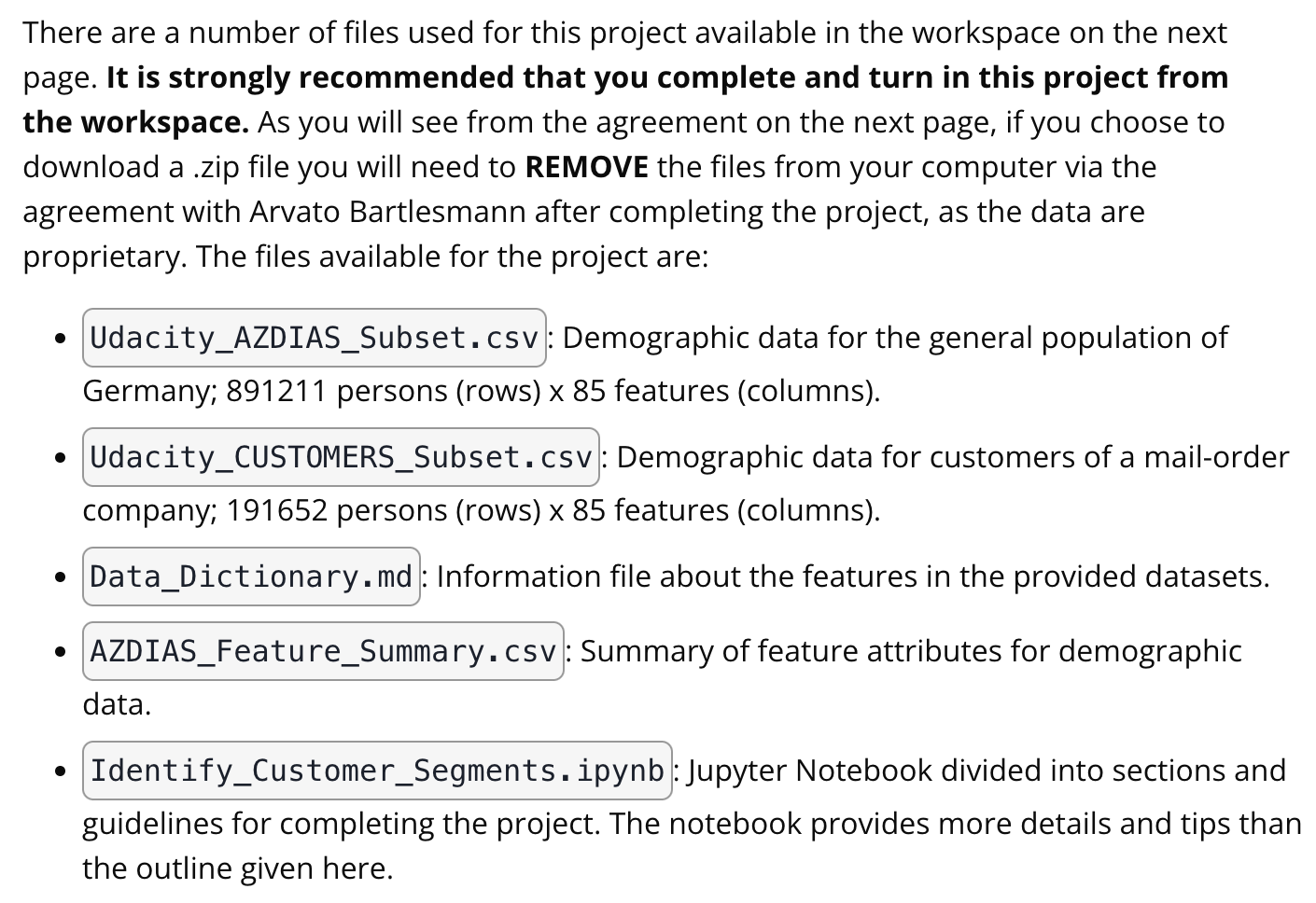
• Missing value in each column

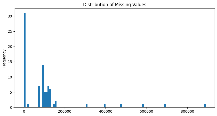
• Missing value in each row

• Split subset of data with missing value with threshold 9 in each row

Discussion:

• We will split the data into two subsets: one for data points that are above 10 for missing values, and a second subset for points below that threshold.
• Compare distribution of values between the two groups. If the distributions of non-missing features look similar between the data with many missing values and the data with few or no missing values, then we could argue that simply dropping those points from the analysis won't present a major issue.
• Remove columns that have more than threshold of missing data.

2. Re-Encode Features

• Re-Encode Categorical Features

binary_columns = df_azdias_categorical.columns[(df_azdias_categorical.nunique() == 2)].tolist()
print("Binary columns: ", binary_columns)
multi_level_columns = df_azdias_categorical.columns[(df_azdias_categorical.nunique() > 2)].tolist()
print("Multi-level columns: ", multi_level_columns)

Then apply one-hot encoding to the binary and multi-level categorical data.

df_azdias_smaller_9_missing = pd.get_dummies(
    data=df_azdias_smaller_9_missing,
    columns=multi_level_columns_new,
    prefix=multi_level_columns_new,
    dtype='int8'
)

• Re-Encode Mixed Features

df_summary[df_summary['type'] == 'mixed']

Then feature engineer the mixed data by Data_Dictionary.md.

Discussion: For the categorical features, I first identified which columns were categorical and separated them into binary variables (with 2 values) and multiple variables.

• The 5 binary categorical features all provide relevant information for forming customer segments, so the decision was made to keep them all, including the non-numerical feature related to the building's location in East or West Germany prior to 1991. This feature may be less useful now than it was 10 or 20 years ago.
• For the multi-categorical variables, each category was analyzed individually:
• The categories CJT_GESAMTTYP, FINANZTYP, NATIONALITAET_KZ, SHOPPER_TYP, and ZABEOTYP all related to person-level features without being too detailed, so the decision was made to keep them and one-hot encode them.
• For LP_FAMILIE_FEIN, LP_FAMILIE_GROB, LP_STATUS_FEIN, and LP_STATUS_GROB, the decision was made to drop the "Grobs" which were summaries of the "Feins". The level of segregation was better for identifying customer segments in the more detailed "Fein" scales, but it was unnecessary to keep both.
• The category GEBAEUDETYP provided no additional value for customer segmentation as it related to building-level features which could be inferred from ANZ_HAUSHALTE_AKTIV, so it was dropped.
• Between CAMEO_DEUG_2015 and CAMEO_DEU_2015, which both relate to wealth/life stage typology, the decision was made to keep only the rough scale of CAMEO_DEUG_2015. CAMEO_DEU_2015 was too detailed for this particular customer segment analysis, and it would be appropriate to use it in a second analysis after primary customer segments have been identified for fine-tuning marketing efforts.
• Lastly, GFK_URLAUBERTYP is a detailed analysis of vacation habits with 12 categories. It was a close choice on whether to keep or drop it for the same reasons discussed above. On balance, it was kept and one-hot encoded because it was a person-level feature.

Feature Transformation

1. Apply Imputation

from sklearn.impute import SimpleImputer

simple_imputer = SimpleImputer()
df = pd.DataFrame(simple_imputer.fit_transform(df))

2. Perform Feature Scaling

from sklearn.preprocessing import StandardScaler

scaler = StandardScaler()
df = pd.DataFrame(scaler.fit_transform(df))

3. PCA

from sklearn.decomposition import PCA

pca = PCA()
df = pd.DataFrame(pca.fit_transform(df))

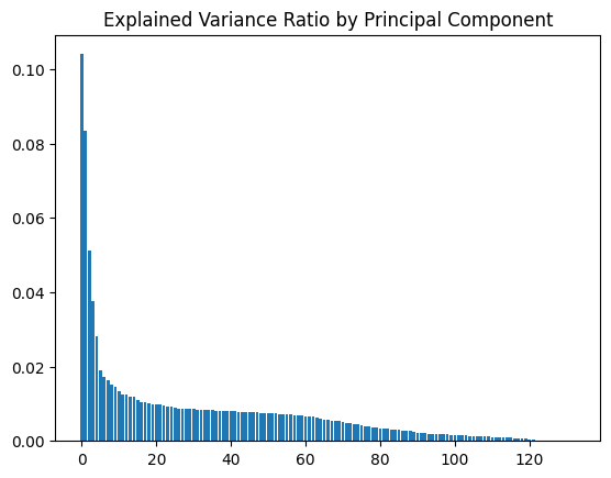
4. Interpret Principal Components

def show_pca_weights(principal_component, number_of_weights):
    ratio = pd.DataFrame(pca.explained_variance_ratio_, columns=['Explained_Variance_Ratio'])
    weights = pd.DataFrame(pca.components_, columns=list(df_azdias_cleaned.columns.values))
    result = pd.concat([ratio, weights], axis=1, sort=False, join='inner')
    print("Principal Component", principal_component, "Weights")
    print(result.iloc[(principal_component)-1].sort_values(ascending=False)[:number_of_weights])

    result = result.sort_values(by='Explained_Variance_Ratio', ascending=False)
    result = result.iloc[principal_component-1:principal_component,1:]
    result = result.transpose()
    result = result.iloc[:number_of_weights,:]
    result = result.iloc[::-1]
    result.plot.barh(figsize=(10,10),legend=False)
    plt.title('Principal Component {} Weights'.format(principal_component))
    plt.xlabel('Weight')
    plt.ylabel('Feature')
    plt.show()

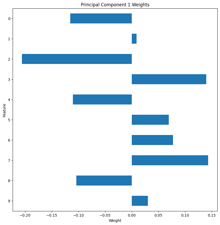
Discussion: I investigated the features by mapping each weight to their corresponding feature name, then sorted the features according to weight. The most interesting features for each principal component, then, were those at the beginning and end of the sorted list.

Clustering

1. Apply Clustering to General Population

from sklearn.cluster import KMeans

kmeans = KMeans(n_clusters=20)
kmeans.fit(df)

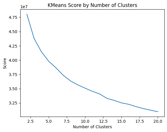
kmeans_20 = KMeans(n_clusters=20, n_init=10, max_iter=100, random_state=8071)
population = kmeans_20.fit_predict(df_pca)

2. Apply Clustering to the Customer Data

customers_cluster = kmeans_20.predict(customers_cleaned)

3. Compare Customer Data to Demographics Data

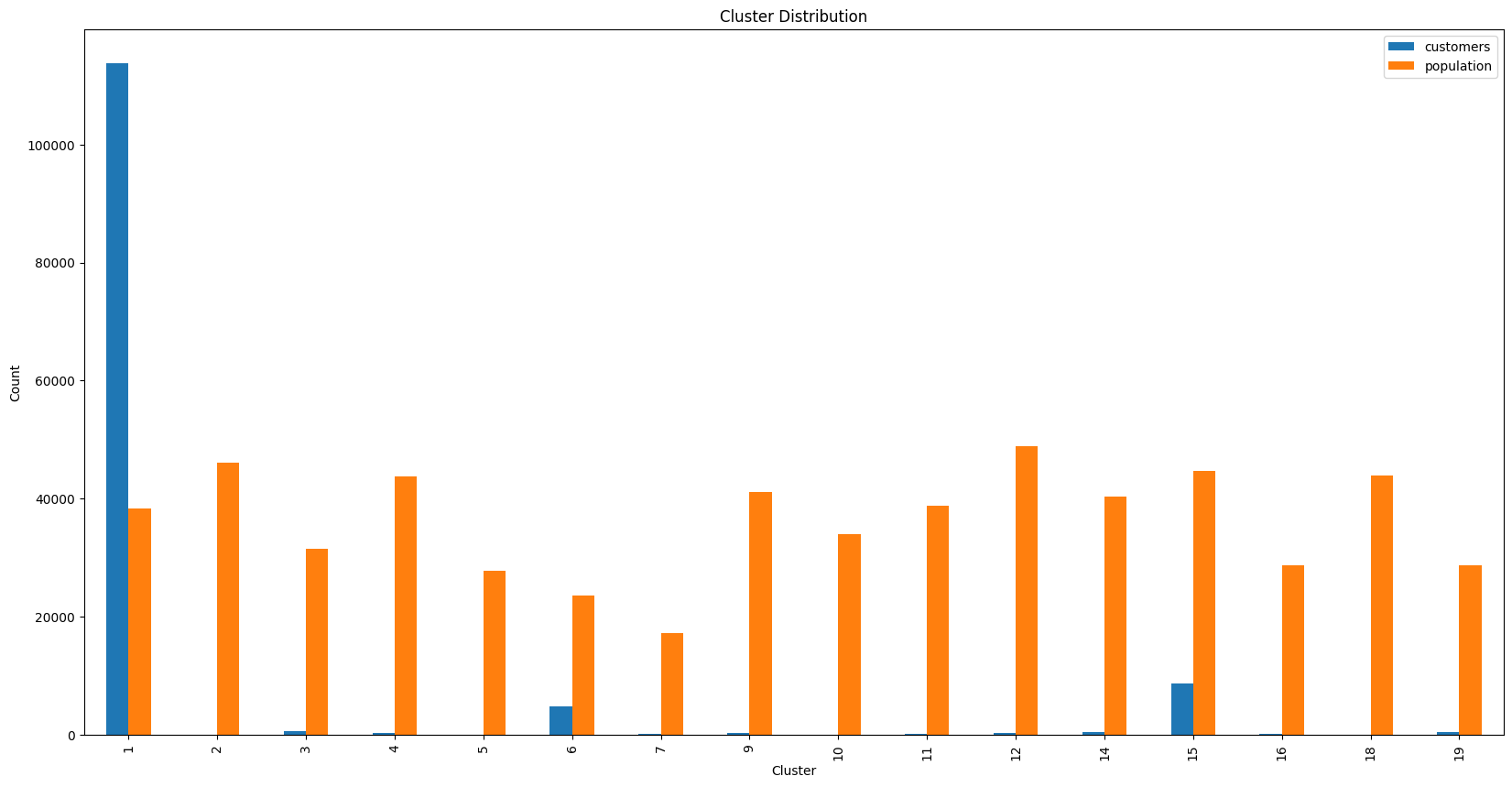
Discussion: I computed the proportion of data points in each cluster for the general population and the customer data. I visualized the ratios in cluster representation between groups. I used Seaborn's countplot() or barplot() function. I also accounted for the number of data points in this subset, for both the general population and customer datasets, when making my computations. I found that cluster 13 is overrepresented in the customer dataset compared to the general population. I inferred that people in this cluster are likely to be older, less wealthy, and less likely to be mainstream consumers. I found that cluster 2 is underrepresented in the customer dataset compared to the general population.

Conclusion

I used unsupervised learning techniques to organize the general population into clusters, then used those clusters to see which of them comprise the main user base for the company. I found that people in cluster 13 are more likely to be customers of the mail-order company, while people in cluster 2 are less likely to be customers of the mail-order company. I also found that people in cluster 13 are likely to be older, less wealthy, and less likely to be mainstream consumers, while people in cluster 2 are likely to be younger, more wealthy, and more likely to be mainstream consumers. The company can use this information to target marketing campaigns towards these two groups accordingly.